Wir alle wissen, dass die gebräuchlichste oder besser gesagt „Standard“-Metrik für die Bewertung von Modellen für tiefes Lernen (insbesondere in Bezug auf die Klassifizierung) derzeit die Accuracy in Bezug auf die Inferenz oder die Time to Accuracy (TTA) in Bezug auf die Training ist. Dies zeigt sich auch in der populärsten Benchmark für maschinelles Lernen namens MLPerf.
Obwohl ResNet das Problem des verschwindenden Gradienten, der in tieferen Architekturen auftritt, gelöst hat und obwohl viele moderne Architekturen (z.B. MobileNet) weniger Parameter benötigen, gibt es einen bedeutenden Kohlenstoff-Fußabdruck für tiefes Lernen. Ein Beispiel hierfür sind die Modelle der natürlichen Sprachverarbeitung, die aufgrund der sehr hohen Anzahl der für das Training benötigten GPUs (z.B. 512 GPUs oder sogar auch 10.000 GPUs) negative Auswirkungen auf die Umwelt haben. Dies ist einer der Hauptgründe, warum die Menschen beginnen, eine grünere KI zu fordern.
 Ich möchte Ihnen meine Forschungsarbeit mit dem Titel „Environmentally-Friendly Metrics for Evaluating the Performance of Deep Learning Models and Systems / Umweltfreundliche Metriken zur Bewertung der Leistung von Modellen und Systemen für das tiefe Lernen“ vorstellen.
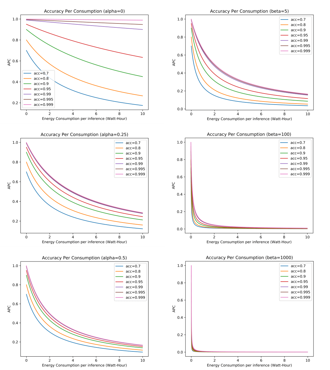
Zusammenfassung: Der Klimawandel gilt als eines der wichtigsten Probleme, mit denen wir derzeit als Spezies konfrontiert sind, und die vorhandenen Metriken und Benchmarks, die zur Bewertung der Leistung verschiedener Deep Learning (DL)-Modelle und -Systeme verwendet werden, konzentrieren sich derzeit hauptsächlich auf ihre Genauigkeit und Geschwindigkeit, ohne auch ihren Energieverbrauch und ihre Kosten zu berücksichtigen. In diesem Papier stellen wir vier neue DL-Metriken vor, zwei bezüglich der Inferenz, die Accuracy Per Consumption (APC) und Accuracy Per Energy Cost (APEC) genannt werden, und zwei bezüglich der Training, die Time to closest APC (TTCAPC) und Time to closest APEC (TTCAPEC) genannt werden, die nicht nur die Genauigkeit eines DL-Modells, sondern auch seinen Energieverbrauch, seine Energiekosten und die Zeit, die für die Training bis zu diesem Punkt benötigt wird, berücksichtigen. Experimentelle Ergebnisse beweisen, dass alle vier DL-Metriken vielversprechend sind, insbesondere diejenige bezüglich der Energiekosten, was zukünftige DL-Forscher dazu ermutigt, bei der Versorgung ihrer DL-basierten Systeme nur grüne Energie zu verwenden.
 Sie können den Artikel hier lesen.


Hier habe ich alle Projektdateien bezüglich unserer Umweltfreundliche Metriken zur Bewertung der Leistung von Modellen und Systemen für tiefes Lernen veröffentlicht.
metric.py
„““
Author: Sorin Liviu Jurj
This is a Python code written for our paper called „Environmentally-Friendly Metrics for Evaluating the Performance of Deep Learning Models and Systems“. More info about this can be found here: https://www.jurj.de/environmentally-friendly-metrics-for-evaluating-the-performance-of-deep-learning-models-and-systems
„““
import numpy as np
import matplotlib.pyplot as plt
def modifiedConsumption(consumption, accuracy, a=0.1):
„““
a is a meassure of the importance of consumption even as the
accuracy goes up
„““
return consumption*((1-a)*(1 – accuracy) + a)
def accuracyPerConsumption(consumption, accuracy, a=0.1, b=1):
„““
ranges from 0 to 1
100% accuracy and 0 consumption returns apc 1
0% accuracy returns apc 0 regardless
apc goes up with accuracy and down with consumption
consumption from innaccurate results is weighted more heavily
„““
return accuracy/(b*modifiedConsumption(consumption, accuracy, a) + 1)
def accuracyPerEnergyCost(energyCost, accuracy, a=0.1, b=1):
„““
ranges from 0 to 1
100% accuracy and 0 cost returns apec 1
0% accuracy returns apec 0 regardless
apec goes up with accuracy and down with consumption
cost from innaccurate results is weighted more heavily
„““
return accuracy/(b*modifiedConsumption(energyCost, accuracy, a) + 1)
accuracies = [0.7, 0.8, 0.9, 0.95, 0.99, 0.995, 0.999]
consumptions = np.arange(0, 10, 0.01)
costs = np.arange(0, 5, 0.05)
betas = [5, 100, 1000]
alphas = [0, 0.25, 0.5]
apcs = []
# Default consumption
# for accuracy in accuracies:
# for consumption in consumptions:
# apc = accuracyPerConsumption(consumption, accuracy, b=1)
# apcs.append(apc)
# plt.plot(consumptions, apcs, label=f“acc={accuracy}“)
# apcs = []
# plt.legend(loc=“best“)
# plt.xlabel(„Energy Consumption per inference (Watt-Hour)“)
# plt.ylabel(„APC“)
# plt.title(f“Accuracy Per Consumption“)
# plt.savefig(„apc_def.png“, dpi=800)
# Default costs
# for accuracy in accuracies:
# for consumption in costs:
# apc = accuracyPerConsumption(consumption, accuracy, b=10)
# apcs.append(apc)
# plt.plot(costs, apcs, label=f“acc={accuracy}“)
# apcs = []
# plt.legend(loc=“best“)
# plt.xlabel(„Energy Cost per inference (cents EUR)“)
# plt.ylabel(„APEC“)
# plt.title(f“Accuracy Per Energy Cost“)
# plt.savefig(„apec_def.png“, dpi=800)
# alpha figures
# for alpha in alphas:
# for accuracy in accuracies:
# for consumption in consumptions:
# apc = accuracyPerConsumption(consumption, accuracy, a=alpha)
# apcs.append(apc)
# plt.plot(consumptions, apcs, label=f“acc={accuracy}“)
# apcs = []
# plt.legend(loc=“best“)
# plt.xlabel(„Energy Consumption per inference (Watt-Hour)“)
# plt.ylabel(„APC“)
# plt.title(f“Accuracy Per Consumption (alpha={alpha})“)
# plt.savefig(f“apc_a{alpha}.png“, dpi=800)
# plt.clf()
# Beta figures
# for beta in betas:
# for accuracy in accuracies:
# for consumption in consumptions:
# apc = accuracyPerConsumption(consumption, accuracy, b=beta)
# apcs.append(apc)
# plt.plot(consumptions, apcs, label=f“acc={accuracy}“)
# apcs = []
# plt.legend(loc=“best“)
# plt.xlabel(„Energy Consumption per inference (Watt-Hour)“)
# plt.ylabel(„APC“)
# plt.title(f“Accuracy Per Consumption (beta={beta})“)
# plt.savefig(f“apc_b{beta}.png“, dpi=800)
# plt.clf()
# Alpha figures (costs)
# for alpha in alphas:
# for accuracy in accuracies:
# for consumption in costs:
# apc = accuracyPerConsumption(consumption, accuracy, a=alpha, b=10)
# apcs.append(apc)
# plt.plot(costs, apcs, label=f“acc={accuracy}“)
# apcs = []
# plt.legend(loc=“best“)
# plt.xlabel(„Energy Cost per inference (cents EUR)“)
# plt.ylabel(„APEC“)
# plt.title(f“Accuracy Per Energy Cost (alpha={alpha})“)
# plt.savefig(f“apec_a{alpha}.png“, dpi=800)
# plt.clf()
# Beta figures (costs)
# for beta in betas:
# for accuracy in accuracies:
# for consumption in costs:
# apc = accuracyPerConsumption(consumption, accuracy, b=beta)
# apcs.append(apc)
# plt.plot(costs, apcs, label=f“acc={accuracy}“)
# apcs = []
# plt.legend(loc=“best“)
# plt.xlabel(„Energy Cost per inference (cents EUR)“)
# plt.ylabel(„APEC“)
# plt.title(f“Accuracy Per Energy Cost (beta={beta})“)
# plt.savefig(f“apec_b{beta}.png“, dpi=800)
# plt.clf()
# Default costs
consumptions = np.arange(0, 20, 0.1)
# for accuracy in accuracies:
# for consumption in consumptions:
# apc = accuracyPerConsumption(consumption, accuracy, b=0.1)
# apcs.append(apc)
# plt.plot(consumptions, apcs, label=f“acc={accuracy}“)
# apcs = []
# values = [(10.4, 0.9056), (10.6, 0.9341), (9.8, 0.9349), (8.88, 0.9454)]
# names = [„VGG-19“, „InceptionV3“, „ResNet-50“, „MobileNetV2″]
# for i, (c, acc) in enumerate(values):
# apc = accuracyPerConsumption(c, acc, b=0.1)
# plt.plot(c, apc, marker=“*“, label=names[i], linestyle=““)
# plt.legend(loc=“best“)
# plt.xlabel(„Energy Consumption per hour (WH)“)
# plt.ylabel(„APC“)
# plt.title(f“Accuracy Per Consumption“)
# plt.savefig(„apc_models.png“, dpi=800)
# plt.clf()
consumptions = np.arange(0, 0.035, 0.001)
wattPrice = 0.00305
for accuracy in accuracies:
for consumption in consumptions:
apc = accuracyPerConsumption(consumption, accuracy, b=50)
apcs.append(apc)
plt.plot(consumptions, apcs)
apcs = []
values = [(10.4, 0.9056), (10.6, 0.9341), (9.8, 0.9349), (8.88, 0.9454)]
names = [„VGG-19“, „InceptionV3“, „ResNet-50“, „MobileNetV2″]
for i, (c, acc) in enumerate(values):
apc = accuracyPerConsumption(c*wattPrice, acc, b=50)
print(apc)
plt.plot(c*wattPrice, apc, marker=“o“, label=names[i]+“ grid powered“, linestyle=““)
for i, (c, acc) in enumerate(values):
c = 0
apc = accuracyPerConsumption(c*wattPrice, acc, b=50)
print(apc)
plt.plot(c*wattPrice, apc, marker=“*“, label=names[i]+“ solar powered“, linestyle=““)
plt.legend(loc=“best“)
plt.xlabel(„Energy Cost per hour (cents EUR)“)
plt.ylabel(„APEC“)
plt.title(f“Accuracy Per Energy Cost“)
plt.savefig(„apec_models.png“, dpi=800)
plt.clf()
metric_with_multiple_points.py
„““
Author: Sorin Liviu Jurj
This is a Python code written for our paper called „Environmentally-Friendly Metrics for Evaluating the Performance of Deep Learning Models and Systems“. More info about this can be found here: https://www.jurj.de/environmentally-friendly-metrics-for-evaluating-the-performance-of-deep-learning-models-and-systems
„““
import numpy as np
import matplotlib.pyplot as plt
def modifiedConsumption(consumption, accuracy, a=0.1):
„““
a is a meassure of the importance of consumption even as the
accuracy goes up
„““
return consumption*((1-a)*(1 – accuracy) + a)
def accuracyPerConsumption(consumption, accuracy, a=0.1, b=1):
„““
ranges from 0 to 1
100% accuracy and 0 consumption returns apc 1
0% accuracy returns apc 0 regardless
apc goes up with accuracy and down with consumption
consumption from innaccurate results is weighted more heavily
„““
return accuracy/(b*modifiedConsumption(consumption, accuracy, a) + 1)
def accuracyPerEnergyCost(energyCost, accuracy, a=0.1, b=1):
„““
ranges from 0 to 1
100% accuracy and 0 cost returns apec 1
0% accuracy returns apec 0 regardless
apec goes up with accuracy and down with consumption
cost from innaccurate results is weighted more heavily
„““
return accuracy/(b*modifiedConsumption(energyCost, accuracy, a) + 1)
accuracies = [0.7, 0.8, 0.9, 0.95, 0.99, 0.995, 0.999]
consumptions = np.arange(0, 10, 0.01)
costs = np.arange(0, 5, 0.05)
betas = [5, 100, 1000]
alphas = [0, 0.25, 0.5]
apcs = []
# Default consumption
# for accuracy in accuracies:
# for consumption in consumptions:
# apc = accuracyPerConsumption(consumption, accuracy, b=1)
# apcs.append(apc)
# plt.plot(consumptions, apcs, label=f“acc={accuracy}“)
# apcs = []
# plt.legend(loc=“best“)
# plt.xlabel(„Energy Consumption per inference (Watt-Hour)“)
# plt.ylabel(„APC“)
# plt.title(f“Accuracy Per Consumption“)
# plt.savefig(„apc_def.png“, dpi=800)
# Default costs
# for accuracy in accuracies:
# for consumption in costs:
# apc = accuracyPerConsumption(consumption, accuracy, b=10)
# apcs.append(apc)
# plt.plot(costs, apcs, label=f“acc={accuracy}“)
# apcs = []
# plt.legend(loc=“best“)
# plt.xlabel(„Energy Cost per inference (cents EUR)“)
# plt.ylabel(„APEC“)
# plt.title(f“Accuracy Per Energy Cost“)
# plt.savefig(„apec_def.png“, dpi=800)
# alpha figures
# for alpha in alphas:
# for accuracy in accuracies:
# for consumption in consumptions:
# apc = accuracyPerConsumption(consumption, accuracy, a=alpha)
# apcs.append(apc)
# plt.plot(consumptions, apcs, label=f“acc={accuracy}“)
# apcs = []
# plt.legend(loc=“best“)
# plt.xlabel(„Energy Consumption per inference (Watt-Hour)“)
# plt.ylabel(„APC“)
# plt.title(f“Accuracy Per Consumption (alpha={alpha})“)
# plt.savefig(f“apc_a{alpha}.png“, dpi=800)
# plt.clf()
# Beta figures
# for beta in betas:
# for accuracy in accuracies:
# for consumption in consumptions:
# apc = accuracyPerConsumption(consumption, accuracy, b=beta)
# apcs.append(apc)
# plt.plot(consumptions, apcs, label=f“acc={accuracy}“)
# apcs = []
# plt.legend(loc=“best“)
# plt.xlabel(„Energy Consumption per inference (Watt-Hour)“)
# plt.ylabel(„APC“)
# plt.title(f“Accuracy Per Consumption (beta={beta})“)
# plt.savefig(f“apc_b{beta}.png“, dpi=800)
# plt.clf()
# Alpha figures (costs)
# for alpha in alphas:
# for accuracy in accuracies:
# for consumption in costs:
# apc = accuracyPerConsumption(consumption, accuracy, a=alpha, b=10)
# apcs.append(apc)
# plt.plot(costs, apcs, label=f“acc={accuracy}“)
# apcs = []
# plt.legend(loc=“best“)
# plt.xlabel(„Energy Cost per inference (cents EUR)“)
# plt.ylabel(„APEC“)
# plt.title(f“Accuracy Per Energy Cost (alpha={alpha})“)
# plt.savefig(f“apec_a{alpha}.png“, dpi=800)
# plt.clf()
# Beta figures (costs)
# for beta in betas:
# for accuracy in accuracies:
# for consumption in costs:
# apc = accuracyPerConsumption(consumption, accuracy, b=beta)
# apcs.append(apc)
# plt.plot(costs, apcs, label=f“acc={accuracy}“)
# apcs = []
# plt.legend(loc=“best“)
# plt.xlabel(„Energy Cost per inference (cents EUR)“)
# plt.ylabel(„APEC“)
# plt.title(f“Accuracy Per Energy Cost (beta={beta})“)
# plt.savefig(f“apec_b{beta}.png“, dpi=800)
# plt.clf()
# Default costs
consumptions = np.arange(0, 20, 0.1)
# for accuracy in accuracies:
# for consumption in consumptions:
# apc = accuracyPerConsumption(consumption, accuracy, b=0.1)
# apcs.append(apc)
# plt.plot(consumptions, apcs, label=f“acc={accuracy}“)
# apcs = []
# values = [(10.4, 0.9056), (10.6, 0.9341), (9.8, 0.9349), (8.88, 0.9454)]
# names = [„VGG-19“, „InceptionV3“, „ResNet-50“, „MobileNetV2″]
# for i, (c, acc) in enumerate(values):
# apc = accuracyPerConsumption(c, acc, b=0.1)
# plt.plot(c, apc, marker=“*“, label=names[i], linestyle=““)
# plt.legend(loc=“best“)
# plt.xlabel(„Energy Consumption per hour (WH)“)
# plt.ylabel(„APC“)
# plt.title(f“Accuracy Per Consumption“)
# plt.savefig(„apc_models.png“, dpi=800)
# plt.clf()
consumptions = np.arange(0, 0.045, 0.001)
wattPrice = 0.00305
# for accuracy in accuracies:
# for consumption in consumptions:
# apc = accuracyPerConsumption(consumption, accuracy, b=50)
# apcs.append(apc)
# plt.plot(consumptions, apcs, label=f“acc={accuracy}“)
# apcs = []
values = [(10.4, 0.9056), (10.6, 0.9341), (9.8, 0.9349), (8.88, 0.9454)]
names = [„VGG-19“, „InceptionV3“, „ResNet-50“, „MobileNetV2″]
# for i, (c, acc) in enumerate(values):
# apc = accuracyPerConsumption(c*wattPrice, acc, b=50)
# print(apc)
# plt.plot(c*wattPrice, apc, marker=“o“, label=names[i]+“ grid powered“, linestyle=““)
# for i, (c, acc) in enumerate(values):
# c = 0
# apc = accuracyPerConsumption(c*wattPrice, acc, b=50)
# print(apc)
# plt.plot(c*wattPrice, apc, marker=“*“, label=names[i]+“ solar powered“, linestyle=““)
# plt.legend(loc=“best“)
# plt.xlabel(„Energy Cost per hour (cents EUR)“)
# plt.ylabel(„APEC“)
# plt.title(f“Accuracy Per Energy Cost“)
# plt.savefig(„apec_models.png“, dpi=800)
# plt.clf()
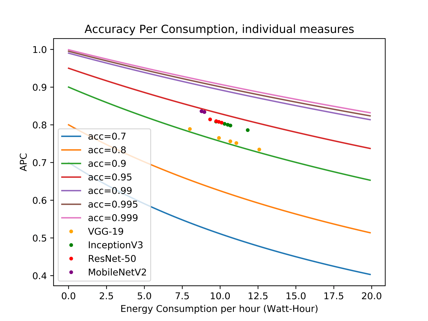
cs = [[11.07, 9.92, 10.67, 8, 12.58],
[10.5, 9.73, 11.82, 10.68, 10.29],
[9.74, 9.34, 9.91, 10.1],
[8.78, 8.77, 8.95, 8.96]]
accs = [0.9056, 0.9341, 0.9349, 0.9454]
colors = [„orange“, „green“, „red“, „purple“]
# for i in range(len(accs)):
# acc = accs[i]
# name = names[i]
# color = colors[i]
# c = cs[i][0]
# apc = accuracyPerConsumption(c*wattPrice, acc, b=50)
# plt.plot(c*wattPrice, apc,
# marker=“.“, linestyle=““, c=color, label=name + “ grid powered“)
# for c in cs[i][1:]:
# apc = accuracyPerConsumption(c*wattPrice, acc, b=50)
# plt.plot(c*wattPrice, apc,
# marker=“.“, label=None, linestyle=““, c=color)
# plt.legend(loc=“best“)
# plt.xlabel(„Energy Cost per hour (cents EUR)“)
# plt.ylabel(„APEC“)
# plt.title(f“Accuracy Per Energy Cost, individual measures“)
# plt.savefig(„apec_models_individual_measures.png“, dpi=800)
# plt.show()
# plt.clf()
consumptions = np.arange(0, 20, 0.1)
for accuracy in accuracies:
for consumption in consumptions:
apc = accuracyPerConsumption(consumption, accuracy, b=0.1)
apcs.append(apc)
plt.plot(consumptions, apcs, label=f“acc={accuracy}“)
apcs = []
for i in range(len(accs)):
acc = accs[i]
name = names[i]
color = colors[i]
c = cs[i][0]
apc = accuracyPerConsumption(c, acc, b=0.1)
plt.plot(c, apc,
marker=“.“, linestyle=““, c=color, label=name)
for c in cs[i][1:]:
apc = accuracyPerConsumption(c, acc, b=0.1)
plt.plot(c, apc,
marker=“.“, label=None, linestyle=““, c=color)
plt.legend(loc=“best“)
plt.xlabel(„Energy Consumption per hour (Watt-Hour)“)
plt.ylabel(„APC“)
plt.title(f“Accuracy Per Consumption, individual measures“)
plt.savefig(„apc_models_individual_measures.png“, dpi=800)
plt.show()
plt.clf()
metric_with_gpu_comparison.py
„““
Author: Sorin Liviu Jurj
This is a Python code written for our paper called „Environmentally-Friendly Metrics for Evaluating the Performance of Deep Learning Models and Systems“. More info about this can be found here: https://www.jurj.de/environmentally-friendly-metrics-for-evaluating-the-performance-of-deep-learning-models-and-systems
„““
import numpy as np
import matplotlib.pyplot as plt
def modifiedConsumption(consumption, accuracy, a=0.1):
„““
a is a meassure of the importance of consumption even as the
accuracy goes up
„““
return consumption*((1-a)*(1 – accuracy) + a)
def accuracyPerConsumption(consumption, accuracy, a=0.1, b=1):
„““
ranges from 0 to 1
100% accuracy and 0 consumption returns apc 1
0% accuracy returns apc 0 regardless
apc goes up with accuracy and down with consumption
consumption from innaccurate results is weighted more heavily
„““
return accuracy/(b*modifiedConsumption(consumption, accuracy, a) + 1)
def accuracyPerEnergyCost(energyCost, accuracy, a=0.1, b=1):
„““
ranges from 0 to 1
100% accuracy and 0 cost returns apec 1
0% accuracy returns apec 0 regardless
apec goes up with accuracy and down with consumption
cost from innaccurate results is weighted more heavily
„““
return accuracy/(b*modifiedConsumption(energyCost, accuracy, a) + 1)
accuracies = [0.7, 0.8, 0.9, 0.95, 0.99, 0.995, 0.999]
consumptions = np.arange(0, 10, 0.01)
costs = np.arange(0, 5, 0.05)
betas = [5, 100, 1000]
alphas = [0, 0.25, 0.5]
apcs = []
# Default consumption
# for accuracy in accuracies:
# for consumption in consumptions:
# apc = accuracyPerConsumption(consumption, accuracy, b=1)
# apcs.append(apc)
# plt.plot(consumptions, apcs, label=f“acc={accuracy}“)
# apcs = []
# plt.legend(loc=“best“)
# plt.xlabel(„Energy Consumption per inference (Watt-Hour)“)
# plt.ylabel(„APC“)
# plt.title(f“Accuracy Per Consumption“)
# plt.savefig(„apc_def.png“, dpi=800)
# Default costs
# for accuracy in accuracies:
# for consumption in costs:
# apc = accuracyPerConsumption(consumption, accuracy, b=10)
# apcs.append(apc)
# plt.plot(costs, apcs, label=f“acc={accuracy}“)
# apcs = []
# plt.legend(loc=“best“)
# plt.xlabel(„Energy Cost per inference (cents EUR)“)
# plt.ylabel(„APEC“)
# plt.title(f“Accuracy Per Energy Cost“)
# plt.savefig(„apec_def.png“, dpi=800)
# alpha figures
# for alpha in alphas:
# for accuracy in accuracies:
# for consumption in consumptions:
# apc = accuracyPerConsumption(consumption, accuracy, a=alpha)
# apcs.append(apc)
# plt.plot(consumptions, apcs, label=f“acc={accuracy}“)
# apcs = []
# plt.legend(loc=“best“)
# plt.xlabel(„Energy Consumption per inference (Watt-Hour)“)
# plt.ylabel(„APC“)
# plt.title(f“Accuracy Per Consumption (alpha={alpha})“)
# plt.savefig(f“apc_a{alpha}.png“, dpi=800)
# plt.clf()
# Beta figures
# for beta in betas:
# for accuracy in accuracies:
# for consumption in consumptions:
# apc = accuracyPerConsumption(consumption, accuracy, b=beta)
# apcs.append(apc)
# plt.plot(consumptions, apcs, label=f“acc={accuracy}“)
# apcs = []
# plt.legend(loc=“best“)
# plt.xlabel(„Energy Consumption per inference (Watt-Hour)“)
# plt.ylabel(„APC“)
# plt.title(f“Accuracy Per Consumption (beta={beta})“)
# plt.savefig(f“apc_b{beta}.png“, dpi=800)
# plt.clf()
# Alpha figures (costs)
# for alpha in alphas:
# for accuracy in accuracies:
# for consumption in costs:
# apc = accuracyPerConsumption(consumption, accuracy, a=alpha, b=10)
# apcs.append(apc)
# plt.plot(costs, apcs, label=f“acc={accuracy}“)
# apcs = []
# plt.legend(loc=“best“)
# plt.xlabel(„Energy Cost per inference (cents EUR)“)
# plt.ylabel(„APEC“)
# plt.title(f“Accuracy Per Energy Cost (alpha={alpha})“)
# plt.savefig(f“apec_a{alpha}.png“, dpi=800)
# plt.clf()
# Beta figures (costs)
# for beta in betas:
# for accuracy in accuracies:
# for consumption in costs:
# apc = accuracyPerConsumption(consumption, accuracy, b=beta)
# apcs.append(apc)
# plt.plot(costs, apcs, label=f“acc={accuracy}“)
# apcs = []
# plt.legend(loc=“best“)
# plt.xlabel(„Energy Cost per inference (cents EUR)“)
# plt.ylabel(„APEC“)
# plt.title(f“Accuracy Per Energy Cost (beta={beta})“)
# plt.savefig(f“apec_b{beta}.png“, dpi=800)
# plt.clf()
# Default costs
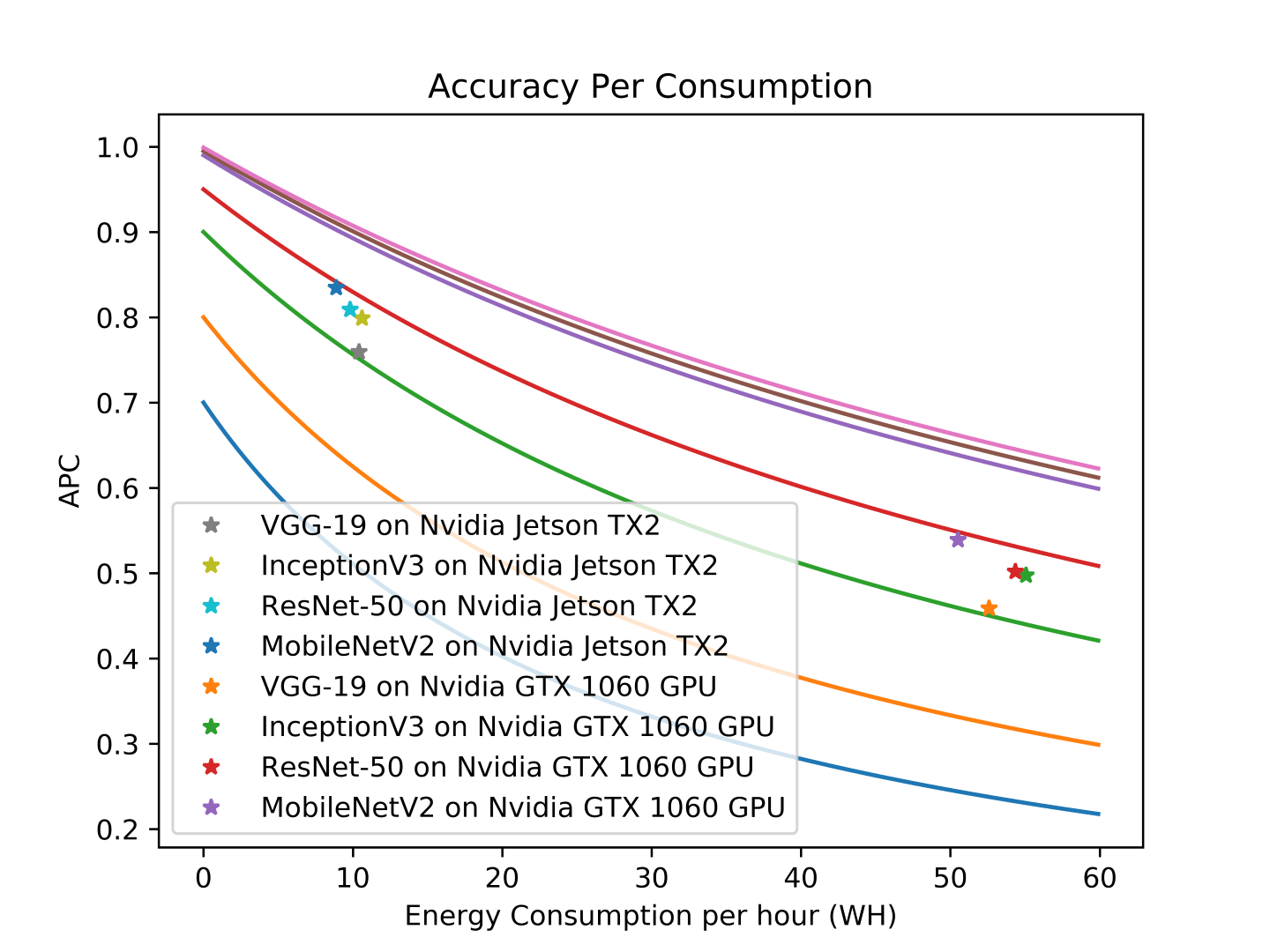
consumptions = np.arange(0, 60, 0.1)
for accuracy in accuracies:
for consumption in consumptions:
apc = accuracyPerConsumption(consumption, accuracy, b=0.1)
apcs.append(apc)
plt.plot(consumptions, apcs)
apcs = []
values = [(10.4, 0.9056), (10.6, 0.9341), (9.8, 0.9349), (8.88, 0.9454),
(52.58, 0.9056), (55.06, 0.9341), (54.35, 0.9349), (50.51, 0.9454)]
names = [„VGG-19 on Nvidia Jetson TX2“,
„InceptionV3 on Nvidia Jetson TX2“,
„ResNet-50 on Nvidia Jetson TX2“,
„MobileNetV2 on Nvidia Jetson TX2“,
„VGG-19 on Nvidia GTX 1060 GPU“,
„InceptionV3 on Nvidia GTX 1060 GPU“,
„ResNet-50 on Nvidia GTX 1060 GPU“,
„MobileNetV2 on Nvidia GTX 1060 GPU“]
for i, (c, acc) in enumerate(values):
apc = accuracyPerConsumption(c, acc, b=0.1)
plt.plot(c, apc, marker=“*“, label=names[i], linestyle=““)
plt.legend(loc=“best“)
plt.xlabel(„Energy Consumption per hour (WH)“)
plt.ylabel(„APC“)
plt.title(f“Accuracy Per Consumption“)
plt.savefig(„apc_models_compared_to_gpu.png“, dpi=800)
plt.show()
plt.clf()
consumptions = np.arange(0, 0.045, 0.001)
wattPrice = 0.00305
# for accuracy in accuracies:
# for consumption in consumptions:
# apc = accuracyPerConsumption(consumption, accuracy, b=50)
# apcs.append(apc)
# plt.plot(consumptions, apcs)
# apcs = []
# values = [(10.4, 0.9056), (10.6, 0.9341), (9.8, 0.9349), (8.88, 0.9454)]
# names = [„VGG-19“, „InceptionV3“, „ResNet-50“, „MobileNetV2″]
# for i, (c, acc) in enumerate(values):
# apc = accuracyPerConsumption(c*wattPrice, acc, b=50)
# print(apc)
# plt.plot(c*wattPrice, apc, marker=“o“, label=names[i]+“ grid powered“, linestyle=““)
# for i, (c, acc) in enumerate(values):
# c = 0
# apc = accuracyPerConsumption(c*wattPrice, acc, b=50)
# print(apc)
# plt.plot(c*wattPrice, apc, marker=“*“, label=names[i]+“ solar powered“, linestyle=““)
# plt.legend(loc=“best“)
# plt.xlabel(„Energy Cost per hour (cents EUR)“)
# plt.ylabel(„APEC“)
# plt.title(f“Accuracy Per Energy Cost“)
# #plt.savefig(„apec_models.png“, dpi=800)
# plt.show()
# plt.clf()
cs = [[11.07, 9.92, 10.67, 8, 12.58],
[10.5, 9.73, 11.82, 10.68, 10.29],
[9.74, 9.34, 9.91, 10.1],
[8.78, 8.77, 8.95, 8.96]]
accs = [0.9056, 0.9341, 0.9349, 0.9454]
colors = [„orange“, „green“, „red“, „purple“]
# for i in range(len(accs)):
# acc = accs[i]
# name = names[i]
# color = colors[i]
# c = cs[i][0]
# apc = accuracyPerConsumption(c*wattPrice, acc, b=50)
# plt.plot(c*wattPrice, apc,
# marker=“.“, linestyle=““, c=color, label=name + “ grid powered“)
# for c in cs[i][1:]:
# apc = accuracyPerConsumption(c*wattPrice, acc, b=50)
# plt.plot(c*wattPrice, apc,
# marker=“.“, label=None, linestyle=““, c=color)
# plt.legend(loc=“best“)
# plt.xlabel(„Energy Cost per hour (cents EUR)“)
# plt.ylabel(„APEC“)
# plt.title(f“Accuracy Per Energy Cost, individual measures“)
# plt.savefig(„apec_models_individual_measures.png“, dpi=800)
# plt.show()
# plt.clf()
# consumptions = np.arange(0, 20, 0.1)
# for accuracy in accuracies:
# for consumption in consumptions:
# apc = accuracyPerConsumption(consumption, accuracy, b=0.1)
# apcs.append(apc)
# plt.plot(consumptions, apcs, label=f“acc={accuracy}“)
# apcs = []
# for i in range(len(accs)):
# acc = accs[i]
# name = names[i]
# color = colors[i]
# c = cs[i][0]
# apc = accuracyPerConsumption(c, acc, b=0.1)
# plt.plot(c, apc,
# marker=“.“, linestyle=““, c=color, label=name)
# for c in cs[i][1:]:
# apc = accuracyPerConsumption(c, acc, b=0.1)
# plt.plot(c, apc,
# marker=“.“, label=None, linestyle=““, c=color)
# plt.legend(loc=“best“)
# plt.xlabel(„Energy Consumption per hour (Watt-Hour)“)
# plt.ylabel(„APC“)
# plt.title(f“Accuracy Per Consumption, individual measures“)
# plt.savefig(„apc_models_individual_measures.png“, dpi=800)
# plt.show()
# plt.clf()
train_metrics.py
„““
Author: Sorin Liviu Jurj
This is a Python code written for our paper called „Environmentally-Friendly Metrics for Evaluating the Performance of Deep Learning Models and Systems“. More info about this can be found here: https://www.jurj.de/environmentally-friendly-metrics-for-evaluating-the-performance-of-deep-learning-models-and-systems
„““
import numpy as np
import matplotlib.pyplot as plt
from metric import accuracyPerConsumption
maxEnergy = np.random.uniform()*1000
maxEnergy = 10
energyDelta = 0.1
accuracyDelta = 0.01
energies = np.arange(0, maxEnergy+energyDelta, energyDelta)
accuracies = np.arange(0, 1, accuracyDelta)
print(energies, accuracies)
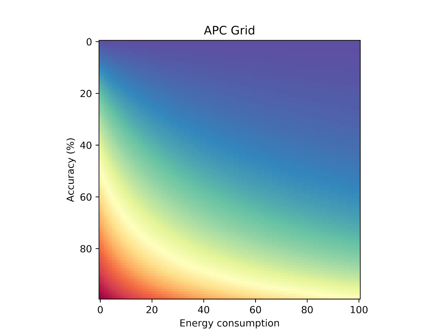
data = np.zeros([len(accuracies), len(energies)])
for i in range(len(accuracies)):
for j in range(len(energies)):
data[i, j] = accuracyPerConsumption(energies[j] + energyDelta*0.5, accuracies[i] + accuracyDelta*0.5)
fig, ax = plt.subplots()
# Using matshow here just because it sets the ticks up nicely. imshow is faster.
ax.imshow(data, cmap=’Spectral_r‘)
# for (i, j), z in np.ndenumerate(data):
# ax.text(j, i, ‚{:0.2f}‘.format(z), ha=’center‘, va=’center‘)
plt.title(„APC Grid“)
plt.xlabel(„Energy consumption“)
plt.ylabel(„Accuracy (%)“)
plt.savefig(„APC Grid 1“, dpi=800)
plt.show()

Neueste Kommentare